Mass GANs

Generative Adversarial Networks (GANs) have enabled significant advances across numerous fields, ranging from art creation to deepfake video generation. The potential of GANs, however, is not restricted to 2D space. The development and application of 3D GANs have opened new possibilities, particularly in the field of design.

This project examines the possibilities of 3D GANs in the design field with the following objectives:

Grasp the fundamental concepts behind GANs and their 3D extension.
Appreciate the power and nuances of 3D GANs through hands-on experiments.
Examine how 3D GANs can be harnessed for product design, architectural modeling, and virtual environment creation.
Visualize and manipulate the latent space to generate novel and innovative designs.
Understand the limitations of current 3D GAN models and the potential areas of improvement.

Generative Adversarial Networks, commonly referred to as GANs, are a class of artificial intelligence algorithms designed to generate new data that resemble a given set of data. The architecture of a GAN consists of two primary components.

1. Generator

The role of the generator is to create fake data.
It takes random noise from a latent space and produces data samples as its output.
The primary objective of the generator is to produce data that is indistinguishable from real data.

2.Discriminator

The discriminator functions as a binary classifier.
It aims to differentiate between real and fake data.
The discriminator receives both real data samples and the fake data generated by the generator, and its task is to correctly label each one as 'real' or 'fake'.

The diagram below illustrates this process, showing how the generator's output is evaluated by the discriminator, resulting in a loss that drives the improvement of both components.

Generative adversarial networks concept diagram

1. Point cloud

A point cloud is a set of data points in space. In 3D shape representation, point clouds are typically used to represent the external surface of an object, and each point in the point cloud has an (x, y, z) coordinate.
A point cloud can represent any 3D shape without being limited to a specific topology or grid (high flexibility).
Points are disconnected, so additional processing is often required to extract surfaces or other features (limited connectivity).

2. Voxel

Voxels (short for volumetric pixels) are the 3D equivalent of 2D pixels. A voxel representation divides the 3D space into a regular grid, and each cell (or voxel) in the grid can be either occupied or empty.
Operations such as convolution are straightforward to apply on voxel grids (simplicity).
Representing fine details requires a very high-resolution grid, which can be computationally prohibitive (limited resolution).

3. Mesh

A 3D mesh consists of vertices, edges, and faces that define the shape of a 3D object in space. The most common type of mesh is a triangular mesh, where the shape is represented using triangles.
A mesh can represent both simple and complex geometries (high expressiveness).
A mesh provides information about how points are connected, which is useful for many applications (continuous surface representation).
Operations on meshes, such as subdivision or simplification, can be computationally demanding (complexity).

First, a practical application is implemented in which a GAN is trained on point cloud data to generate a single sphere represented as a point cloud. Before the neural networks are implemented, the target sphere point cloud is loaded from a file. A single sphere shape was modeled using Rhino.

Normalization is particularly beneficial when the training data consists of similar objects in various sizes, or when the absolute size is not critical for the task. For the dataset of a single sphere, the absolute size is not significant, so the data is normalized. The sphere can be normalized easily using numpy as follows:


    class Normalize:
        def __call__(self, pointcloud):
            assert len(pointcloud.shape) == 2
            
            norm_pointcloud = pointcloud - np.mean(pointcloud, axis=0) 
            norm_pointcloud /= np.max(np.linalg.norm(norm_pointcloud, axis=1))
            
            return norm_pointcloud

When different 3D models have different numbers of vertices, sampling a consistent number of points from each model ensures that the input size remains uniform. This is essential when feeding data to neural networks that expect a consistent input size. The code related to PointSampler is available at the following link.

Simple implementation: A single sphere GAN

A sphere, represented by point cloud
From the left, original sphere · random sampled sphere · normalized and random sampled sphere

The data preprocessing is now complete, and the data is ready for model training. A model comprising a simple generator and discriminator is defined and trained as follows:


    class Generator(nn.Module):
        def __init__(self, input_dim=3, output_dim=3, hidden_dim=128):
            super(Generator, self).__init__()
            self.fc1 = nn.Linear(input_dim, hidden_dim)
            self.fc2 = nn.Linear(hidden_dim, hidden_dim)
            self.fc3 = nn.Linear(hidden_dim, hidden_dim)
            self.fc4 = nn.Linear(hidden_dim, output_dim)
    
        def forward(self, x):
            x = torch.relu(self.fc1(x))
            x = torch.relu(self.fc2(x))
            x = torch.relu(self.fc3(x))
            x = torch.tanh(self.fc4(x))
            
            return x
    
    class Discriminator(nn.Module):
        def __init__(self, input_dim=3, hidden_dim=128):
            super(Discriminator, self).__init__()
            self.fc1 = nn.Linear(input_dim, hidden_dim)
            self.fc2 = nn.Linear(hidden_dim, hidden_dim)
            self.fc3 = nn.Linear(hidden_dim, hidden_dim)
            self.fc4 = nn.Linear(hidden_dim, 1)
    
        def forward(self, x):
            x = torch.relu(self.fc1(x))
            x = torch.relu(self.fc2(x))
            x = torch.relu(self.fc3(x))
            x = torch.sigmoid(self.fc4(x))
            
            return x

The complete code, which includes the generator, discriminator, data handling, and training process, can be found at the following link. The training process, visualized using Matplotlib, is shown below. The loss status graph indicates that a sphere begins to form around the 2700-epoch mark. Beyond this point, the loss values stop oscillating and exhibit a convergent graph.

Training process of a single sphere GAN
From the left, losses status · generated point cloud sphere

Implementing the fundamentals and a single sphere GAN above provides a working understanding of GANs. Building on this understanding, the model is now trained with buildings (Masses) designed by architects in order to create a generator that produces fake Masses.

The implementation of MassGAN follows the processes below:

Preparation and preprocessing of the dataset.
Implementation and training of the models.
Evaluation of the generator and exploration of the latent space.

Building models designed by several renowned architects were collected for model training. The figure below shows the actual buildings corresponding to the modeling data that was gathered.

Preparation and preprocessing of the dataset

Voxel-shaped buildings
From the left, RED7(MVRDV architects) · 79 and Park(BIG architects) · Mountain dwelling(BIG architects)

The buildings mentioned above share a common characteristic: a voxel-shaped configuration. As described above, three modalities of 3D shape representation relevant to GANs were introduced. The primary limitation of the voxel-shaped representation is its difficulty in articulating high resolution. Within architectural design, however, this constraint can be reconsidered as an opportunity. The voxel-shaped form is widely used in the architecture field, and there is no strong demand for high-resolution depictions of such forms.

Accordingly, a generative model is created that produces masses similar to those described above, using voxel data at appropriate resolutions. First, to train models from the modeling data, the data structure must be transformed from the .obj format to the more suitable .binvox format. The .binvox format represents data as a binary voxel grid structure, encoding True (1) for solid regions and False (0) for vacant spaces. An illustrative example preprocessed into the .binvox format is shown below.

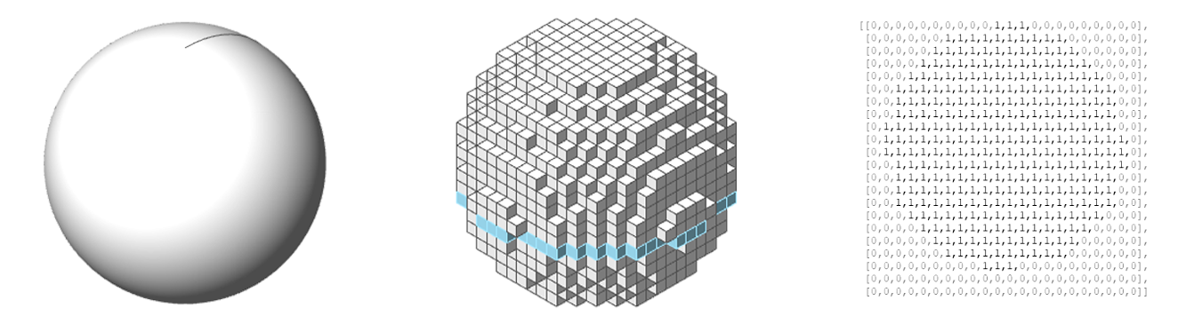Binary voxel grid representations From the left, Given sphere · Voxelated sphere · Binary voxel grid(9th voxels grid) These… — Binary voxel grid representations
From the left, Given sphere · Voxelated sphere · Binary voxel grid(9th voxels grid)
These were described in a previous post titled Voxelate

As shown above in the binary voxel grid, the vacant regions are represented by 0s, while the solid regions are denoted by 1s. The complete preprocessing code for the .binvox format is provided in the following link, and it was used to preprocess the 6 models below to a 32 x 32 x 32 resolution.

(Initially, 24 models had been curated for training MassGAN. However, due to the limited computational performance of the RTX 3060 laptop graphics card, which resulted in prolonged training durations, the dataset size was reduced.)

Preprocessed data to the binary voxel grid utilizing binvox From the top left, 79 and Park · Lego tower, RED7 From the… (1 of 2) — Preprocessed data to the binary voxel grid utilizing binvox
From the top left, 79 and Park · Lego tower, RED7
From the bottom left, Vancouver house · CCTV Headquarter, Mountain dwelling

Preprocessed data to the binary voxel grid utilizing binvox From the top left, 79 and Park · Lego tower, RED7 From the… (2 of 2) — Preprocessed data to the binary voxel grid utilizing binvox
From the top left, 79 and Park · Lego tower, RED7
From the bottom left, Vancouver house · CCTV Headquarter, Mountain dwelling

The procedures for data collection and preprocessing are now complete. The next step is the implementation of both the generator and the discriminator.

DCGAN was implemented with reference to GitHub repositories in which several 3D generation models are implemented, as follows. The complete code defining the models can be accessed at the following link: massGAN/model.py


    class Generator(nn.Module, Config):
        def __init__(self, z_dim, init_out_channels: int = None):
            super().__init__()
            
            out_channels_0 = self.GENERATOR_INIT_OUT_CHANNELS if init_out_channels is None else init_out_channels
            out_channels_1 = int(out_channels_0 / 2)
            out_channels_2 = int(out_channels_1 / 2)

            self.main = nn.Sequential(
                nn.ConvTranspose3d(z_dim, out_channels_0, kernel_size=4, stride=1, padding=0, bias=False),
                nn.BatchNorm3d(out_channels_0),
                nn.ReLU(True),
                nn.ConvTranspose3d(out_channels_0, out_channels_1, kernel_size=4, stride=2, padding=1, bias=False),
                nn.BatchNorm3d(out_channels_1),
                nn.ReLU(True),
                nn.ConvTranspose3d(out_channels_1, out_channels_2, kernel_size=4, stride=2, padding=1, bias=False),
                nn.BatchNorm3d(out_channels_2),
                nn.ReLU(True),
                nn.ConvTranspose3d(out_channels_2, 1, kernel_size=4, stride=2, padding=1, bias=False),
                nn.Sigmoid()
            )
            
            self.to(self.DEVICE)
            
        def forward(self, x):
            return self.main(x)
        
        
    class Discriminator(nn.Module, Config):
        def __init__(self, init_out_channels: int = None):
            super().__init__()
            
            out_channels_0 = self.DISCRIMINATOR_INIT_OUT_CHANNELS if init_out_channels is None else init_out_channels
            out_channels_1 = out_channels_0 * 2
            out_channels_2 = out_channels_1 * 2

            self.main = nn.Sequential(
                nn.Conv3d(1, out_channels_0, kernel_size=4, stride=2, padding=1, bias=False),
                nn.LeakyReLU(0.2, inplace=True),
                nn.Conv3d(out_channels_0, out_channels_1, kernel_size=4, stride=2, padding=1, bias=False),
                nn.BatchNorm3d(out_channels_1),
                nn.LeakyReLU(0.2, inplace=True),
                nn.Conv3d(out_channels_1, out_channels_2, kernel_size=4, stride=2, padding=1, bias=False),
                nn.BatchNorm3d(out_channels_2),
                nn.LeakyReLU(0.2, inplace=True),
                nn.Conv3d(out_channels_2, 1, kernel_size=4, stride=1, padding=0, bias=False),
                nn.Sigmoid()
            )
            
            self.to(self.DEVICE)
            
        def forward(self, x):
            return self.main(x).view(-1, 1).squeeze(1)

In addition, the MassganTrainer was defined for model supervision, including model training, evaluation, and storage. Throughout this process, any issues arising during the training phase were monitored. The recorded outcomes are presented below:

Visualized training process at each 200 epochs from 0 to 20000 From the top, losses status · generated masses when training… (1 of 2) — Visualized training process at each 200 epochs from 0 to 20000
From the top, losses status · generated masses when training model

Visualized training process at each 200 epochs from 0 to 20000 From the top, losses status · generated masses when training… (2 of 2) — Visualized training process at each 200 epochs from 0 to 20000
From the top, losses status · generated masses when training model

In contrast to the a single sphere GAN trained previously, MassGAN does not exhibit a loss value that converges to a single point, owing to the complexity of the data. Nevertheless, a comparison between the early and final stages of training shows that the loss value oscillates within a low range. Furthermore, the monitored fake masses progressively approximate the shapes of the real masses.

The parameters for model training, such as learning rate, batch size, noise dimension, and so forth, were used as follows:


    class ModelConfig:
        """Configuration related to the GAN models
        """

        DEVICE = "cpu"
        if torch.cuda.is_available():
            DEVICE = "cuda"
            
        SEED = 777
        
        GENERATOR_INIT_OUT_CHANNELS = 256
        DISCRIMINATOR_INIT_OUT_CHANNELS = 64
        
        EPOCHS = 20000
        LEARNING_RATE = 0.0001
        BATCH_SIZE = 6
        BATCH_SIZE_TO_EVALUATE = 6
        Z_DIM = 128
        BETAS = (0.5, 0.999)
        
        LAMBDA_1 = 10
        
        LOG_INTERVAL = 200

The model trained with the corresponding ModelConfig is now loaded and evaluated. In a GAN, it is important to evaluate the model quantitatively through the status of the loss, but qualitatively evaluating the data produced by the Generator is also an effective means of evaluation. The following figures show masses generated by the MassGAN model through the evaluate function.

Generated masses by MassGAN model (1 of 6) — Generated masses by MassGAN model

Generated masses by MassGAN model (2 of 6) — Generated masses by MassGAN model

Overall, the model appears to produce reasonable data. Next, several of the masses created by the generator are selected in order to observe the interpolation of latent mass shapes between them.