Wave function collapse is a quantum mechanics concept
where a system in a superposition of states
instantly reduces to a single, definite state upon measurement or observation.
In computer science, the Wave Function Collapse (WFC) algorithm is a technique for generating procedural,
constraint-based content, such as tilemaps or textures, similar to solving a 3D Sudoku puzzle.
Each cell in a grid is initially treated as a superposition of all possible states.
Rather than sampling all cells simultaneously, WFC proceeds by selecting a single cell,
collapsing its state space to one concrete value, and then propagating the resulting constraints to neighboring cells.
 Intuition of how the WFC algorithm works
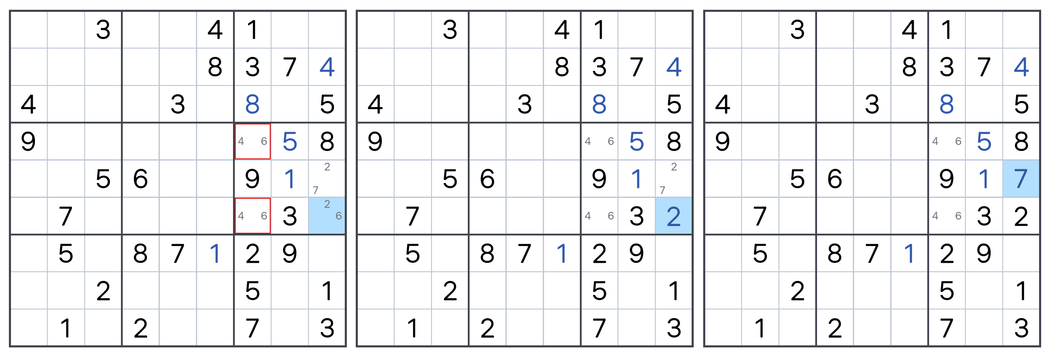
Consider first the 3x3 block in the right-center of the leftmost image.
Each cell in this area has two candidate numbers, and the red cells all share the same candidates ($4, 6$).
Because the red cells must be filled with either $4$ or $6$,
the state of the blue cell is forced to collapse to $2$; otherwise, a contradiction would occur.
After the blue cell collapses to $2$, the cell directly above it, which has $2$ and $7$ as candidates, collapses to $7$.
To apply WFC to real-world design, the abstract states must be turned into concrete, connectable blocks.
The algorithm then operates on a finite set of such modules. Each module is defined by how it can attach to its neighbors, so that collapse and propagation remain purely rule-based.
A natural reference is modular systems, in which a small set of physical pieces combine in many ways under clear connection rules.
LYCS's Modular CATable is one such example: a limited set of table segments with defined interfaces can be rearranged into different table layouts. This idea translates directly into a 3D tileset for WFC.
Inspired by this kind of modular design, I defined the 3D tileset for WFC.
Each tile is a block with six faces ($\pm x$, $\pm y$, $\pm z$), and each face
carries an interface label.
Two neighboring tiles are compatible only if their touching faces carry compatible labels (6-way compatibility). The algorithm propagates constraints using these rules rather than the geometry itself.
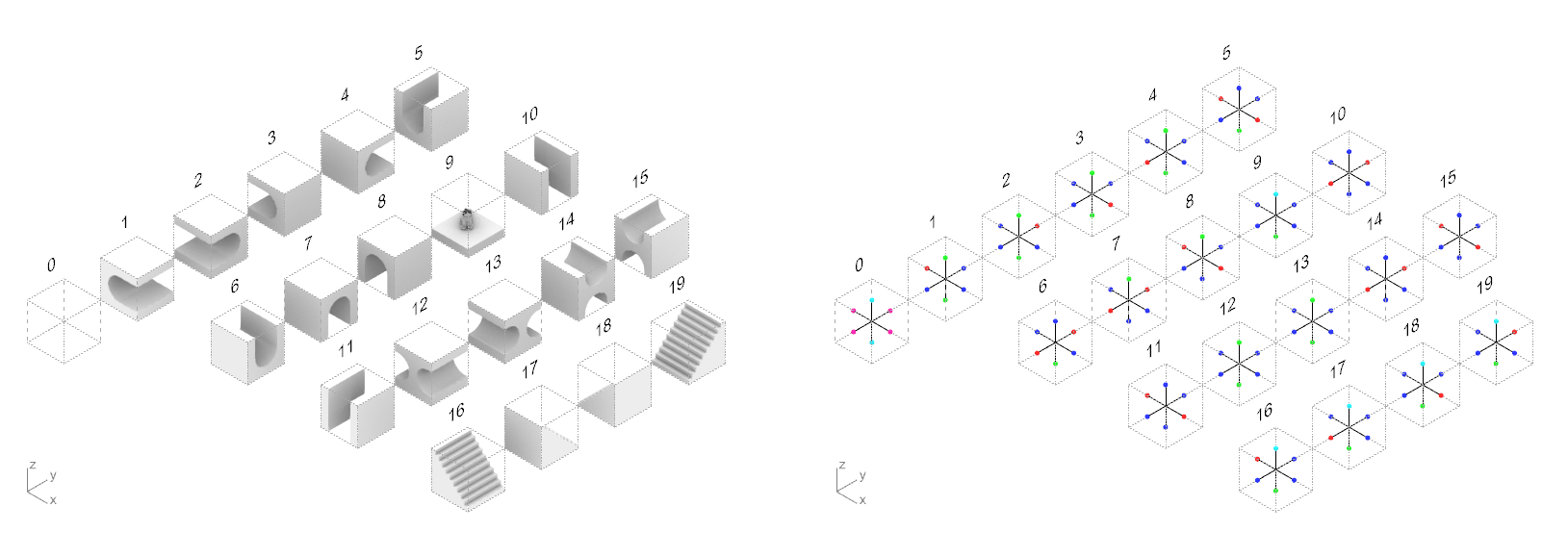
The left panel of the figure below shows the 3D tileset, and the right panel shows the compatibility visualization.
In the right panel, the six dots per cube represent one label per face, color-coded, and the allowed adjacencies follow from compatible labels on touching faces.
For example, tiles $6$ and $7$ are compatible across their $+z$ and $-z$ faces.
Because the $+z$ face of $6$ is OPEN and the $-z$ face of $7$ is OPEN, the two tiles are compatible.
 3D tileset and compatibility visualization
In code, the tileset is stored as a Python dictionary
INTERFACE:
each key is a tile ID from $0$ to $19$, and each value is a mapping from the six face directions ($\pm x$, $\pm y$, $\pm z$) to one of five
labels—
FREE,
OPEN,
CLOSED,
SUPPORT, and
EMPTY.
Tile $0$ is the empty cell. Tiles $1$–$19$ are the solid building blocks.
Compatibility between neighboring tiles is determined by these labels: for any pair of touching faces, the labels must match,
except that
FREE acts as a wildcard and is compatible with any label on the adjacent face.
The snippet below shows the relevant constants and a subset of
INTERFACE from
wfc.py.
    class WaveFunctionCollapseInterface:
        XP = "+x"
        XN = "-x"
        YP = "+y"
        YN = "-y"
        ZP = "+z"
        ZN = "-z"

        FREE = "free"
        OPEN = "open"
        CLOSED = "closed"
        SUPPORT = "support"
        EMPTY = "empty"

        TILE_SIZE = 1

        (...)

        INTERFACE = {
            0: {
                XP: FREE,
                XN: FREE,
                YP: FREE,
                YN: FREE,
                ZP: EMPTY,
                ZN: EMPTY,
            },
        (...)

        17: {
            XP: OPEN,
            XN: OPEN,
            YP: OPEN,
            YN: CLOSED,
            ZP: EMPTY,
            ZN: SUPPORT,
        },
        18: {
            XP: CLOSED,
            XN: OPEN,
            YP: OPEN,
            YN: OPEN,
            ZP: EMPTY,
            ZN: SUPPORT,
        },
        19: {
            XP: OPEN,
            XN: OPEN,
            YP: CLOSED,
            YN: OPEN,
            ZP: EMPTY,
            ZN: SUPPORT,
        },
    }
The grid state is held in a single 4D boolean tensor
states of shape $(H, D, W, T)$, where $T = 20$ is the number of tiles.
A value of
True at
states[z, y, x, t] means tile $t$ is still a candidate for cell $(x, y, z)$.
Collapse and propagation then reduce to bitmask updates on this tensor.
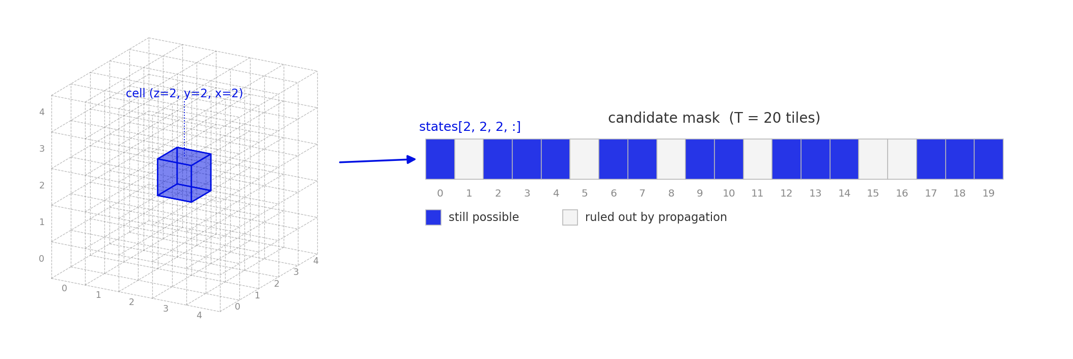 Each grid cell carries a 20-bit candidate mask; propagation only ever flips True bits to False
Compatibility is precomputed once. For every direction $d$, a $T \times T$ boolean matrix
compatibility[d] stores which tile pairs are allowed across that face.
The matrix is built by iterating over every ordered pair of tiles, looking up the labels on the touching faces
(the face $d$ of the first tile against the opposite face of the second), and applying the rule:
in the horizontal directions a
FREE label is a wildcard, and otherwise the two labels must match exactly.
    def _compute_compatibility(self) -> Dict[str, torch.Tensor]:
        compatibility = {}
        for direction in self.directions:
            compatibility_matrix = torch.zeros(
                (len(self.tiles), len(self.tiles)), dtype=torch.bool
            )
            direction_opposite = self.opposite[direction]

            for tile_a in self.tiles:
                tile_a_index = self.tile_to_index[tile_a]
                tile_a_label = self.INTERFACE[tile_a][direction]

                for tile_b in self.tiles:
                    tile_b_index = self.tile_to_index[tile_b]
                    tile_b_label = self.INTERFACE[tile_b][direction_opposite]

                    compatibility_matrix[tile_a_index, tile_b_index] = (
                        self._is_compatible(tile_a_label, tile_b_label, direction)
                    )

            compatibility[direction] = compatibility_matrix

        return compatibility
Because of how the rule is defined, the matrices satisfy
compatibility["+x"] == compatibility["-x"].t() and the same for $\pm y$ and $\pm z$ — propagation in one direction
is the transpose of propagation in the opposite direction.
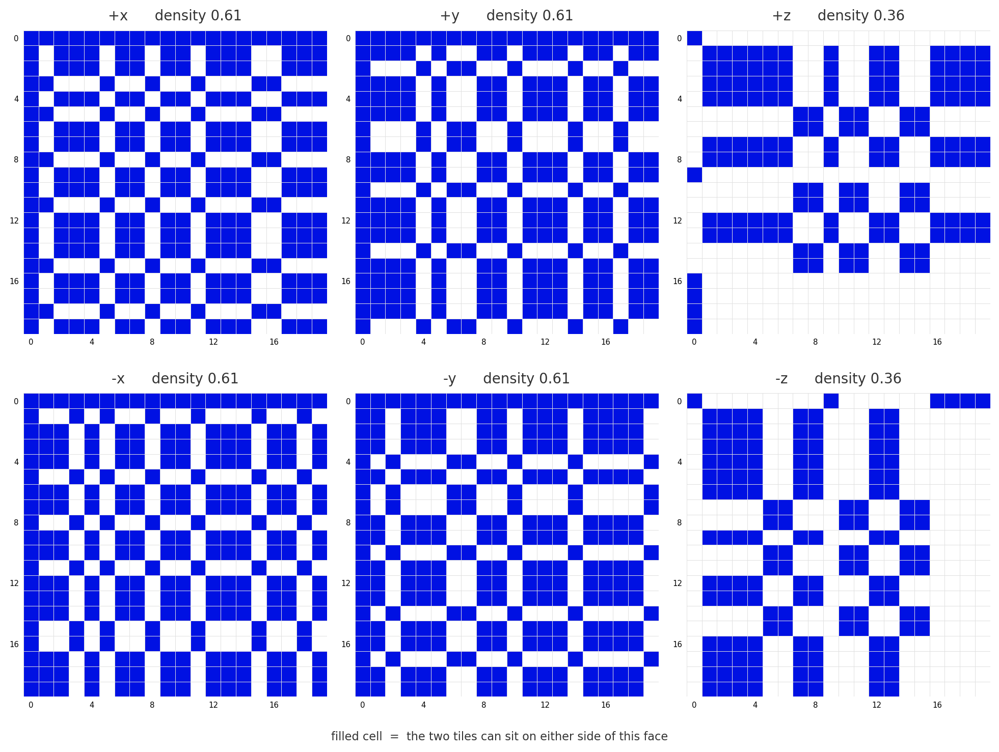 The six $20 \times 20$ compatibility matrices. The horizontal directions $\pm x, \pm y$ are denser ($\approx 0.61$ allowed pairs) because
 FREE acts as a wildcard; the vertical $\pm z$ matrices are sparser ($\approx 0.36$) because $\pm z$ requires an exact label match. The horizontal pairs are transposes of each other.
A cell collapses by drawing one tile from its current candidate set. The candidates are converted to a float vector,
multiplied element-wise by
cell_weights, and passed to
torch.multinomial.
The only weight that differs from $1$ is the entry for tile $0$ (the empty tile),
which is scaled by the user-controlled
empty_weight.
A value below $1$ favors dense structures, while a value above $1$ produces sparser, more open shapes.
    def _collapse(self, x: int, y: int, z: int) -> bool:
        states_int = self.states[z, y, x, :].float()
        states_int *= self.cell_weights

        tile_index_to_collapse = torch.multinomial(
            states_int / states_int.sum(), 1
        ).item()

        self.states[z, y, x, :] = False
        self.states[z, y, x, tile_index_to_collapse] = True

        propagation_status = self._propagate(x=x, y=y, z=z)

        return propagation_status
After a cell is fixed, the constraints must flow outward. Propagation is a BFS over the grid: a queue is seeded with the just-collapsed cell,
and for each cell pulled off the queue, the algorithm determines, for each of the six neighbors, which of the neighbor's candidates remain reachable given the current candidate set.
The reachable set is the OR of the relevant rows of the compatibility matrix, intersected with the neighbor's existing candidate mask.
If that intersection shrinks the neighbor, the neighbor is pushed back onto the queue.
If it shrinks to nothing, propagation reports failure and the run is reset.
    def _propagate(self, x: int, y: int, z: int) -> bool:
        queue = deque()
        queue.append((x, y, z))

        while queue:
            x, y, z = queue.popleft()
            possible_tiles = self.states[z, y, x, :]

            if not possible_tiles.any():
                return False

            for direction in self.directions:
                dx, dy, dz = self.step[direction]
                ax, ay, az = x + dx, y + dy, z + dz

                if (
                    ax < 0 or ax >= self.width
                    or ay < 0 or ay >= self.depth
                    or az < 0 or az >= self.height
                ):
                    continue

                possible_neighbors = self._get_possible_neighbors(
                    possible_tiles, direction
                )

                before = self.states[az, ay, ax, :]
                after = before & possible_neighbors

                if not after.any():
                    return False

                if torch.all(before == after):
                    continue

                self.states[az, ay, ax, :] = after
                queue.append((ax, ay, az))

        return True
Choosing which cell to collapse next is a separate concern.
_get_min_k_cell
scans the grid and returns the cell with the smallest candidate count greater than one — the lowest-entropy cell.
If any cell has been reduced to zero candidates the function returns
False, signalling a contradiction;
if every cell is already collapsed it returns
None and the run terminates.
The full run loop combines the four primitives — collapse, propagate, min-entropy selection, and reset.
Starting from a user-supplied seed cell $(x_0, y_0, z_0)$, the algorithm repeats the following: collapse the current cell;
if propagation fails or the next selection reports a contradiction, clear the grid and restart from the seed;
otherwise advance to the lowest-entropy cell. The loop terminates when every cell holds exactly one tile, or after
max_iters attempts.
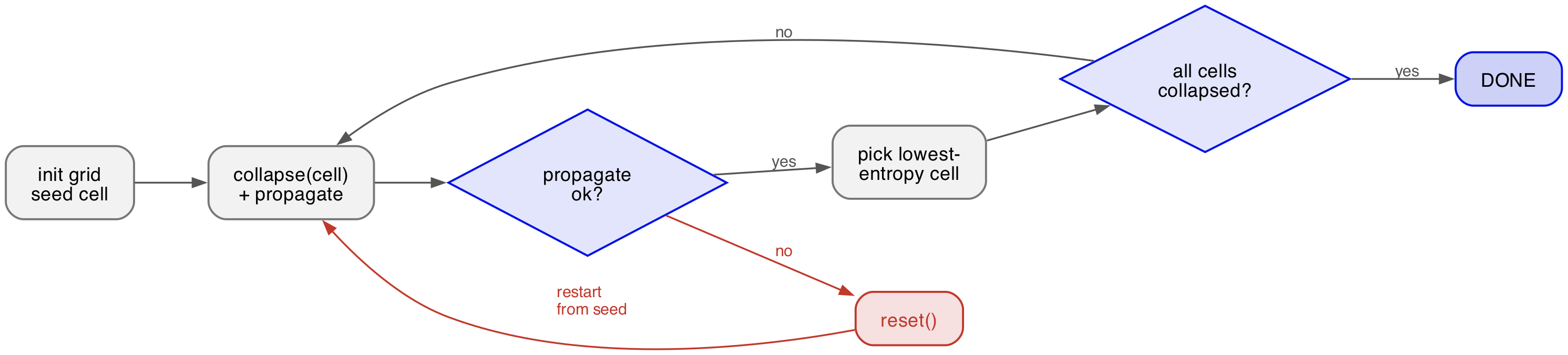 Run loop control flow. The red path is the failure escape: any propagation failure or zero-candidate cell jumps back to the seed.
\[
\begin{array}{l}
\textbf{Algorithm: } \text{Wave Function Collapse 3D}
\end{array}
\]
\[
\begin{array}{l}
\textbf{Input: } W, D, H, \text{ seed cell } (x_0, y_0, z_0), w_{\text{empty}}, \text{max_iters} \\
\textbf{Output: } \text{collapsed grid of tiles}
\end{array}
\]
\[
\begin{array}{l}
\text{Precompute } \mathbf{C}_d \in \{0, 1\}^{T \times T} \text{ for each direction } d \in \{\pm x, \pm y, \pm z\} \\
\texttt{states}[z, y, x, t] \leftarrow 1 \quad \forall (x, y, z, t) \\
\texttt{cell} \leftarrow (x_0, y_0, z_0) \\
\textbf{for } i = 1 \ldots \text{max_iters} \textbf{ do} \\
\quad \textbf{if all cells collapsed: break} \\
\quad \textbf{if not Collapse}(\texttt{cell}) \textbf{ then } \text{Reset}; \texttt{cell} \leftarrow (x_0, y_0, z_0); \textbf{ continue} \\
\quad \texttt{cell} \leftarrow \text{GetMinKCell}() \\
\quad \textbf{if } \texttt{cell} = \text{False} \textbf{ then } \text{Reset}; \texttt{cell} \leftarrow (x_0, y_0, z_0); \textbf{ continue} \\
\quad \textbf{if } \texttt{cell} = \text{None} \textbf{ then break}
\end{array}
\]
\[
\begin{array}{l}
\texttt{Collapse}(x, y, z): \\
\quad t \sim \text{Multinomial}\big(\texttt{states}[z, y, x] \cdot \texttt{cell_weights}\big) \\
\quad \texttt{states}[z, y, x] \leftarrow \mathbf{e}_t \\
\quad \textbf{return Propagate}(x, y, z)
\end{array}
\]
\[
\begin{array}{l}
\texttt{Propagate}(x, y, z): \\
\quad Q \leftarrow \{(x, y, z)\} \\
\quad \textbf{while } Q \neq \emptyset \textbf{ do} \\
\qquad (x, y, z) \leftarrow Q.\text{pop}() \\
\qquad \textbf{for } d \in \{\pm x, \pm y, \pm z\} \textbf{ do} \\
\qquad \quad (x', y', z') \leftarrow \text{neighbor in direction } d \\
\qquad \quad \texttt{valid} \leftarrow \bigvee_{t \,:\, \texttt{states}[z, y, x, t] = 1} \mathbf{C}_d[t, :] \\
\qquad \quad \texttt{after} \leftarrow \texttt{states}[z', y', x'] \wedge \texttt{valid} \\
\qquad \quad \textbf{if not after.any(): return False} \\
\qquad \quad \textbf{if } \texttt{after} \neq \texttt{states}[z', y', x'] \textbf{ then } \texttt{states}[z', y', x'] \leftarrow \texttt{after}; \, Q.\text{push}((x', y', z')) \\
\quad \textbf{return True}
\end{array}
\]
Two design choices govern the behavior of this loop. First, the next cell to collapse is always the one with the fewest remaining candidates,
rather than a random cell. Selecting the lowest-entropy cell concentrates work where the constraints are tightest, which keeps the
set of reachable contradictions small. Second, the failure recovery is deliberately minimal: any contradiction discards
the entire grid and restarts from the same seed cell, with no backtracking or local repair.
For a small grid and a well-designed tileset this is fast enough, whereas on larger grids the cost of repeated full restarts becomes the dominant runtime concern.
The seed is also where directional bias enters. The cat-tower target requires growth from the floor upward, so the seed is fixed at $z_0 = 0$,
and propagation naturally fans outward and upward through the support-bearing tiles. The empty tile (id $0$) acts as a release valve:
raising
empty_weight lets the algorithm select "no tile" more often, producing thinner, more sculptural shapes,
while lowering it forces denser packings.
The frames below are intermediate
.obj snapshots saved during a single run and replayed in order.
Each new frame corresponds to one collapse-and-propagate step, so the animation traces the BFS as it
sweeps outward from the seed cell at the floor. Different runs use different grid sizes, seeds, and
empty_weight values, which is why the resulting cat-towers exhibit such different silhouettes.
Two WFC runs: collapse order on the left, finished structure on the right of each pair