

]]>
~300ms have elapsed
@media (prefers-reduced-motion: reduce), freeze the shimmer to a static gray. The pattern still works without animation
aria-busy="true" to the loading region and remove it on completion. The visual analogue of "loading" should also reach screen-reader users
mouseenter event, replacing the intended tooltip with an unrelated one.
The result is a frustrating flicker effect.
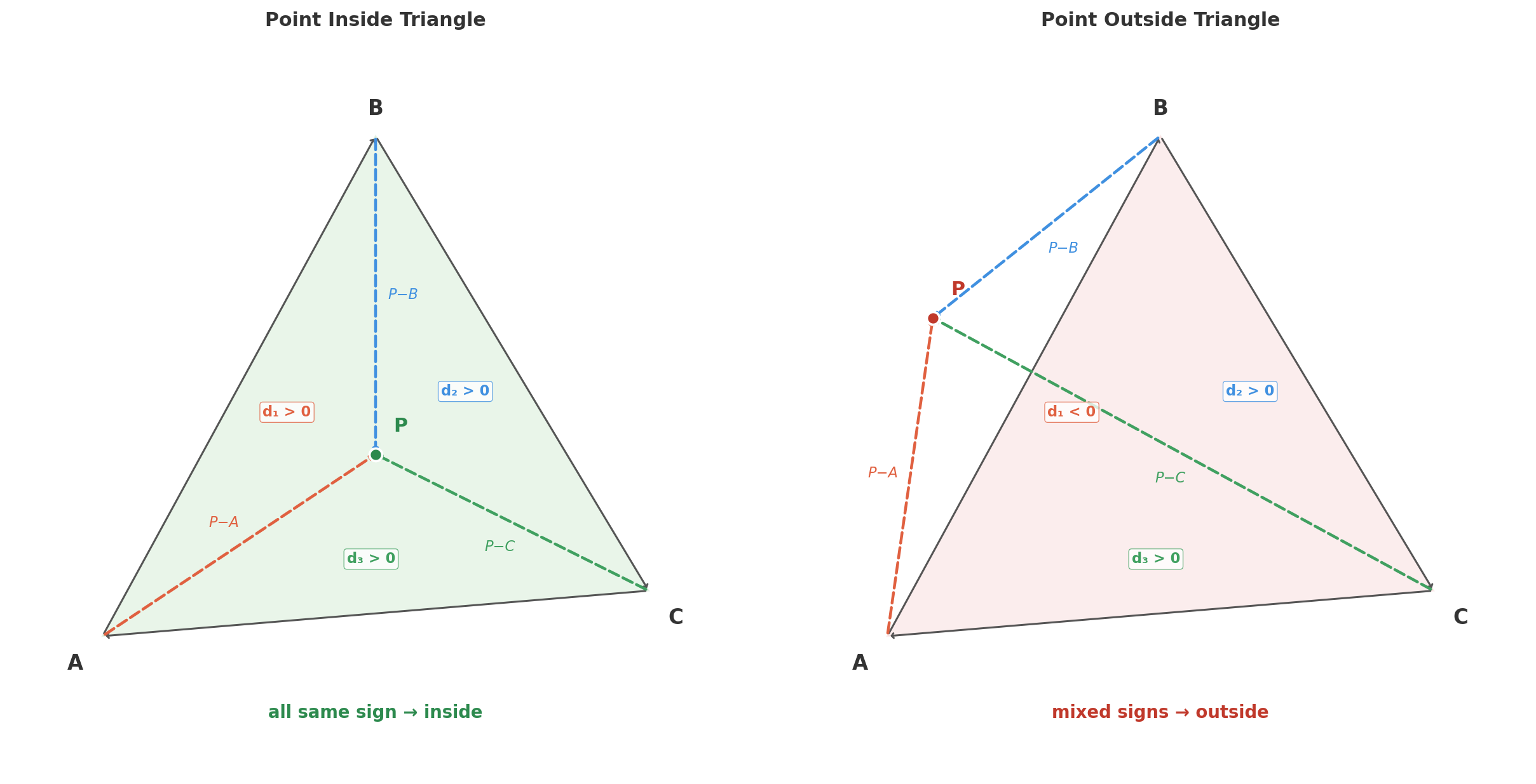
tri_sign function computes this 2D cross product:
    function tri_sign(x1, y1, x2, y2, x3, y3) {
        return (x1 - x3) * (y2 - y3) - (x2 - x3) * (y1 - y3);
    }

    function point_in_triangle(px, py, ax, ay, bx, by, cx, cy) {
        var d1 = tri_sign(px, py, ax, ay, bx, by);
        var d2 = tri_sign(px, py, bx, by, cx, cy);
        var d3 = tri_sign(px, py, cx, cy, ax, ay);
        return !((d1 < 0 || d2 < 0 || d3 < 0) && (d1 > 0 || d2 > 0 || d3 > 0));
    }
!(has_negative && has_positive),
which is true only when all signs agree.
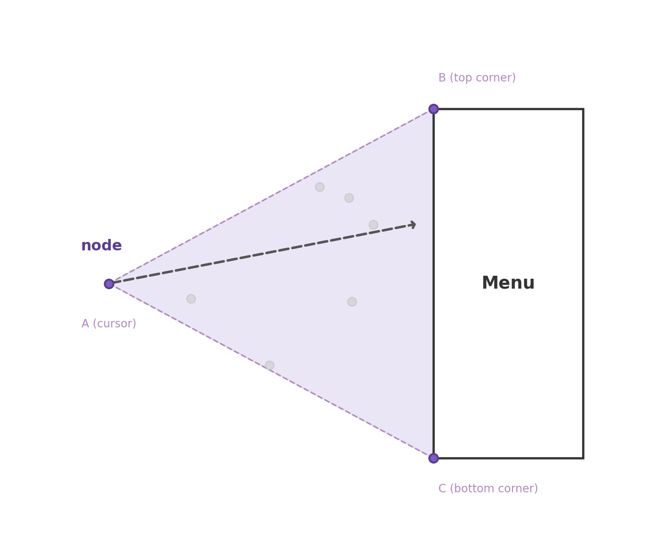
    function build_intent_triangle() {
        // ... get node screen position (dot_x, dot_y)
        // ... get tooltip rect (tt_left, tt_top, tt_w, tt_h)
        var pad = 6;
        return {
            ax: dot_x, ay: dot_y,
            bx: tt_left < dot_x ? tt_left - pad : tt_left + tt_w + pad,
            by: tt_top - pad,
            cx: tt_left < dot_x ? tt_left - pad : tt_left + tt_w + pad,
            cy: tt_top + tt_h + pad
        };
    }
mouseleave on a node:
The system builds the intent triangle and starts a short timer (80ms).
If the cursor reaches the tooltip before the timer fires,
the tooltip's own mouseenter cancels the dismiss.
mouseenter on a different node:
Before activating the new node, the system checks
is_moving_toward_tooltip(mx, my).
If the cursor is inside the intent triangle,
the new node's hover is suppressed, and the current tooltip remains.
    // inside mouseenter handler
    if (intent_triangle && active_hover_node && active_hover_node !== d) {
        var rect = container.getBoundingClientRect();
        var mx = event.clientX - rect.left;
        var my = event.clientY - rect.top;
        if (is_moving_toward_tooltip(mx, my)) return;  // suppress
    }
posted/2026.json)
and auto-generates the repo's README.md papers table.
minute hour day month weekday).
schedule trigger exposes the same syntax to run workflows on a recurring basis.
This bot is set to fire daily at UTC 21:30 (KST 06:30).
workflow_dispatch is also enabled for manual runs.
    on:
      schedule:
        - cron: '30 21 * * *'  # 06:30 KST daily
      workflow_dispatch:
posted/ and README.md.
git diff --staged --quiet skips the commit when there are no changes.
    - name: Save posted history
      run: |
        git config user.name "github-actions"
        git config user.email "actions@github.com"
        git add posted/ README.md
        git diff --staged --quiet || git commit -m "chore: update posted history"
        git push
GEMINI_API_KEY and SLACK_WEBHOOK_URL.
The workflow uses permissions: contents: write to push directly from the action.
/api/daily_papers?date=YYYY-MM-DD
and takes the top result, falling back up to 3 previous days if the date is empty.
down position and its current position:
    protected get isCrossingSelect(): boolean {
        if (!this.rect) return false;
        return this.rect.currentX < this.rect.clientX;
    }
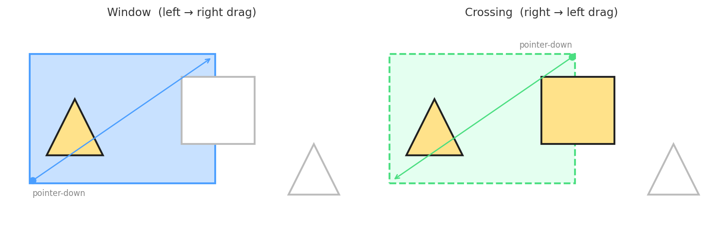
div appended to the main window
on pointerdown and removed on pointerup.
The visual style flips on every pointermove based on the drag direction —
window mode draws a solid blue border with a translucent blue fill,
while crossing mode switches to a dashed green border with a lighter fill,
giving the user the same visual cue they would see in AutoCAD:
    protected updateRect(rect: SelectionRect, event: PointerEvent) {
        if (this.pointerEventMap.size !== 1) return;
        rect.currentX = event.clientX;
        rect.element.style.display = "block";
        const [x1, y1] = [Math.min(rect.clientX, event.clientX), Math.min(rect.clientY, event.clientY)];
        const [x2, y2] = [Math.max(rect.clientX, event.clientX), Math.max(rect.clientY, event.clientY)];
        const crossing = event.clientX < rect.clientX;
        Object.assign(rect.element.style, {
            left: `${x1}px`,
            top: `${y1}px`,
            width: `${x2 - x1}px`,
            height: `${y2 - y1}px`,
            borderStyle: crossing ? "dashed" : "solid",
            backgroundColor: crossing ? "rgba(74, 255, 158, 0.15)" : "rgba(74, 158, 255, 0.3)",
            borderColor: crossing ? "var(--success-color, #4ade80)" : "var(--primary-color)",
        });
    }
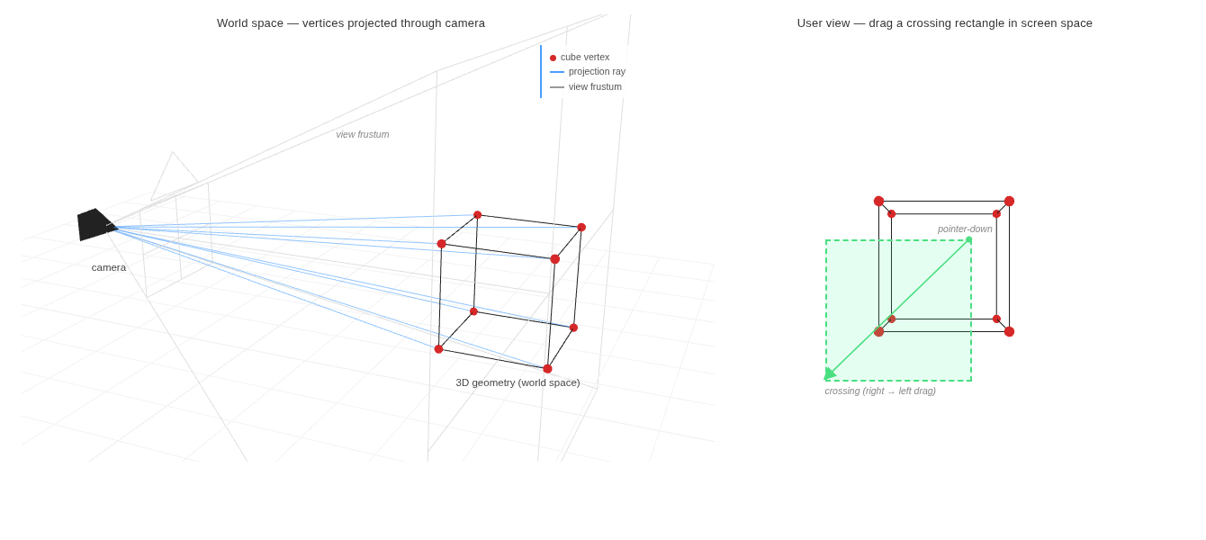
worldToScreen,
producing a 2D point cloud and an edge list.
The mode then selects between two completely different tests.
    private allPointsInsideRect(pts, minX, minY, maxX, maxY): boolean {
        for (const p of pts) {
            if (p.x < minX || p.x > maxX || p.y < minY || p.y > maxY) return false;
        }
        return pts.length > 0;
    }
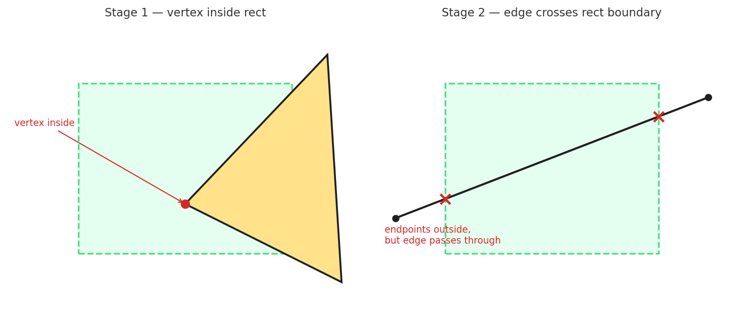
    private anyCrossingHit(pts, edges, minX, minY, maxX, maxY): boolean {
        // 1) any vertex inside rect
        for (const p of pts) {
            if (p.x >= minX && p.x <= maxX && p.y >= minY && p.y <= maxY) return true;
        }
        // 2) any geometry edge crosses rect boundary
        const rectEdges = [
            [minX, minY, maxX, minY],
            [maxX, minY, maxX, maxY],
            [maxX, maxY, minX, maxY],
            [minX, maxY, minX, minY],
        ];
        for (const [ai, bi] of edges) {
            const pa = pts[ai], pb = pts[bi];
            for (const [ex1, ey1, ex2, ey2] of rectEdges) {
                if (segmentsIntersect(pa.x, pa.y, pb.x, pb.y, ex1, ey1, ex2, ey2)) return true;
            }
        }
        return false;
    }
    function segmentsIntersect(x1, y1, x2, y2, x3, y3, x4, y4): boolean {
        const dx1 = x2 - x1, dy1 = y2 - y1;
        const dx2 = x4 - x3, dy2 = y4 - y3;
        const denom = dx1 * dy2 - dy1 * dx2;
        if (Math.abs(denom) < 1e-10) return false;
        const t = ((x3 - x1) * dy2 - (y3 - y1) * dx2) / denom;
        const u = ((x3 - x1) * dy1 - (y3 - y1) * dx1) / denom;
        return t >= 0 && t <= 1 && u >= 0 && u <= 1;
    }
worldToScreen collapses the standard graphics pipeline —
view transform, projection, perspective divide, viewport remap —
into a single helper:
    worldToScreen(point: XYZ): XY {
        const cx = this.width / 2;
        const cy = this.height / 2;
        const vec = new Vector3(point.x, point.y, point.z).project(this.camera);
        return new XY({ x: Math.round(cx * vec.x + cx), y: Math.round(-cy * vec.y + cy) });
    }
Vector3.project(camera) applies the camera's
view matrix \(M_{\text{view}}\) and projection matrix \(M_{\text{proj}}\),
then performs the perspective divide.
The result is in normalized device coordinates (NDC) —
a unit cube where each axis lies in \([-1,\, 1]\):
Object3D start in local space —
each object has its own coordinate frame.
localToWorld applies the object's matrixWorld,
bringing local vertices into the shared world frame
that worldToScreen expects:
    private projectGeometry(obj: Object3D) {
        // ...
        const v = new Vector3();
        const pts: { x: number; y: number }[] = [];
        for (let i = 0; i < posAttr.count; i++) {
            v.fromBufferAttribute(posAttr, i);                // local-space vertex
            obj.localToWorld(v);                              // local → world
            pts.push(this.worldToScreen({ x: v.x, y: v.y, z: v.z }));
        }
        // ...
    }
position buffer attribute,
with the edge list reconstructed from the geometry type
(LineSegments pairs vertices, Line chains them,
Mesh uses the index buffer to build triangle edges).
LineSegments2) are special-cased:
their geometry doesn't store a position attribute at all.
Instead each segment's start and end are stored separately
in instanceStart and instanceEnd instanced attributes,
so the projection has to read both attributes side-by-side and emit them as alternating points.
Without this branch, fat-line edges silently never appear in any rectangle selection.
detectVisualRect) is what runs for
whole-object picks like "select these parts."
For sub-shape picks — selecting individual edges or faces of a B-Rep —
the code delegates to three.js's built-in
SelectionBox,
which performs a true 3D frustum test against the scene:
    detectShapesRect(shapeType, mx1, my1, mx2, my2, ...) {
        // Shape-level rect selection uses SelectionBox for both modes
        // (crossing/window distinction is handled at visual level)
        const selectionBox = this.initSelectionBox(mx1, my1, mx2, my2);
        const detecteds: VisualShapeData[] = [];
        for (const obj of selectionBox.select()) {
            this.addDetectedShape(detecteds, ..., shapeType, obj, ...);
        }
        return detecteds;
    }
SelectionBox builds a frustum from the camera and the two NDC corners
of the drag rectangle, then walks the scene graph and keeps any object whose
bounding volume falls inside.
It doesn't itself distinguish window from crossing —
that distinction is handled one layer up,
where the screen-space projection has finer control over each vertex.
localStorage, it can store large amounts of structured data (objects, files, Blobs, etc.)
localStorage: stores strings only, ~5-10MB max, synchronous API
sessionStorage: similar to localStorage but scoped per tab — data is deleted when the tab/window closes
IndexedDB: can store objects, hundreds of MB or more, asynchronous API
~/.config/google-chrome/Default/IndexedDB/~/Library/Application Support/Google/Chrome/Default/IndexedDB/%LOCALAPPDATA%\Google\Chrome\User Data\Default\IndexedDB\~/.mozilla/firefox/<profile>/storage/default/~/Library/Containers/com.apple.Safari/Data/Library/WebKit/WebsiteData/Default/https_example.com_0.indexeddb.leveldb/
    const estimate = await navigator.storage.estimate();
    console.log(`Used: ${estimate.usage} bytes`);
    console.log(`Quota: ${estimate.quota} bytes`);
await navigator.storage.persist()keyPath or autoIncrement
readonly, readwrite, versionchange
indexedDB.open(name, version)
const request = indexedDB.open("MyDatabase", 1);
onupgradeneeded event
    request.onupgradeneeded = (event) => {
        const db = event.target.result;
        const store = db.createObjectStore("users", { keyPath: "id" });
        store.createIndex("name", "name", { unique: false });
    };
    request.onsuccess = (event) => {
        const db = event.target.result;
        const tx = db.transaction("users", "readwrite");
        const store = tx.objectStore("users");
        store.add({ id: 1, name: "Park", age: 30 });
    };
    const tx = db.transaction("users", "readonly");
    const store = tx.objectStore("users");
    const getRequest = store.get(1);
    getRequest.onsuccess = () => {
        console.log(getRequest.result); // { id: 1, name: "Park", age: 30 }
    };
onsuccess and onerror callbacks
async/await pattern
    import { openDB } from "idb";

    const db = await openDB("MyDatabase", 1, {
        upgrade(db) {
            db.createObjectStore("users", { keyPath: "id" });
        },
    });

    await db.add("users", { id: 1, name: "Park", age: 30 });
    const user = await db.get("users", 1);
onupgradeneeded fires on initial database creation or when the version number is incremented.
Be careful with version management when modifying existing Object Stores
navigator.storage.estimate() to check available capacity
.wasm binary via Emscripten
.js) that handles loading and binding
.wasm, exported functions become callable from JS
emcc (C/C++) or em++ (forces C++ mode), produces .js (glue) + .wasm (binary)
.delete() on Embind class instances — forgetting causes memory leaks
SharedArrayBuffer / pthreads
SharedArrayBuffer + COOP/COEP headers